3 Important Probabilities for Leveraged ETF Investors

In Leveraged ETF and CPPI type Strategy by Bertrand and Prigent I came across an interesting formula: probability of leveraged ETF declining in value while regular fund increases.

Over a period of one day correlation between returns is close to one, but over longer time periods funds usually diverge significantly, that it return of leveraged fund is not leverage times regular funds return. Particularly disappointing situation for leveraged ETF investor is when over some period of time regular ETF increases in value while leveraged ETF declines.
------------------------------------------------
Example 1: consider SSO - ProShares Ultra (leverage_factor=+2) S&P 500 ETF. SPY volatility is about 20%. Expense ratio for SPY is 0.09%, for SPXU 0.91%. I don't know the short rate for SPY but let's assume it is zero. If investor is bullish on the S&P 500 and decided to buy SSO and hold it for 1/2 year, there is 3.31% chance that SSO ill decline even if the investor is correct in the forecast (SPY increases). Even for a relatively short time period on one month such probability is 1.36%.
------------------------------------------------
The formula by Bertrand and Prigent is based on assumption of continuous brownian motion, and is fairly accurate approximation for discrete process. The formula they derived works only for positive leverage, but not for inverse ETFs. I derive formulas for inverse ETFs and also extend their work for different drift conditions, like expense ratios.

The applet below is interactive, but may be a bit slow to update. You can download the spreadsheet on your computer by clicking on Excel button.


Inputs are: leverage factor (negative for inverse ETFs), time in years, volatility of regular ETF (leveraged ETF will have volatility times |leverage|), financing rate, and two drift parameters (for example annual expense ratio of 1% would be -1% drift) Leveraged ETFs usually have higher expense ratios, so I separated the two parameters.

Outputs are: reg pos lev neg - probability that regular ETF will have positive return while leveraged ETF will have a negative return, reg pos lev neg (inv) - same for inverse ETFs, and reg neg lev neg (inv) - probability that both funds decline in value. The reason for two formulas for inverse ETFs is that inverse ETF is "expected" to decline when regular ETF rises in value. Last probability is the disappointing scenario of regular ETF declining, and inverse ETF declining as well.
------------------------------------------------
Example 2: consider SPXU - UltraShort (leverage_factor=-3) S&P 500 ETF. SPY volatility is about 20%. Expense ratio for SPY is 0.09%, for SPXU 0.93%. I don't know the short rate for SPY but let's assume it is zero. If investor is bearish on the S&P 500 and decided to buy SPXU and hold it for 1/2 year, there is 11.77% chance that SPXU will decline even if the investor is correct in the forecast (SPY declines as well). Even for a relatively short time period on one month such probability is non-trivial 4.83%.
------------------------------------------------
Financing cost is the cost to the ETF provider to create leverage - borrow rate for positive leverage ETFs, and short rate for inverse ETFs. I assume that (like in the current environment) one would have to pay both.

cost = IF(leverage_factor>0,rate*(1-leverage_factor)*time,rate*(leverage_factor)*time)

Terms in B9, B10, and B11 are generalized from Bertrand and Prigent's paper. First result is theirs as well, the last two are my contribution.

If you are using the formulas on your blog, website, or research please acknowledge the original source.


Leveraged ETFs Research: Volatility Skew

I have blogged before about inverse and leveraged ETFs, about how their performance depends on their volatility, and also about pricing options on these ETFs. While I try to focus specifically on original research, here are some important research publications from academia, along with my comments.

Volatility skew of leveraged and inverse ETFs is a topic that is dear to my heart - I recently left a trading firm that specializes in volatility arbitrage in ETF space, where over the past year I conducted mathematical research and developed software to create a comprehensive trading system. It is now in production on (almost) all US optionable ETFs. Unfortunately my contract prevents me from disclosing any details about my own research.

1 Dr Jian Zhang thesis, which I believe is the first publication to address correct pricing of LEFT options. I wrote about shortcomings of his three approaches in my previous post.

2 Consistent Pricing of Options on Leveraged ETFs by Andrew Ahn, et al, first provides an important generalization for pricing LEFT options, applying it to Heston model, and also 2 jumps models via Monte-Carlo. They show experimentally model-dependency (that results from path-dependency) for pricing LEFT options.

3 Most recent, is Implied Volatility of Leveraged ETF Options by Tim Leung and Ronnie Sircar. They apply stochastic volatility-based iv asymptotics framework developed in Multiscale Stochastic Volatility for Equity, Interest Rate, and Credit Derivatives, which is an excellent book! Authors also address the issue of different volatility premiums across related products.

4 Structural Slippage of Leveraged ETFs by Doris Dobi and Marco Avellaneda "shows" that you can make money by shorting ETFs and capitalizing on slippage. Despite their findings I don't this that there are any serious money to be made here - 1 borrowing costs are collected from a retail, not institutional broker, 2 actual borrowing costs are not known until stock settles, 3 execution slippage is usually highest at the time of greatest ETF decay. 

Leveraged ETFs Decay And Symmetric vs Skewed Distributions

It has been already widely discussed that LEFT do not decay in the conventional sense like for example options. As a simple thought experiment consider an options that has non-zero Θ even when underlying is not changing in price. Unlike options, LEFTs will not move if underlying ETF or index does not move. The reason why we usually observe downward drift in leveraged ETFs is due to mean-median divergence, and I will try to provide an intuitive explanation of this phenomenon without unnecessary mathematical formulas.

The only working assumption that I will use is that the asset price distribution is "fair", i.e. its expected value tomorrow is it's price today. Also, purely for illustration purposes I made up an ETF with leverage = 1.5 to better show how properties change as leverage factor is increased.

Many people have a mental model of ETF prices changes as a fair process - something like 50% chance it will go up a dollar tomorrow, 50% chance it will fall down a dollar - or some kind of symmetric price distribution.


As leverage and volatility increase, distribution becomes wider, as greater range of prices is possible. However any symmetric distribution of prices has one major problem - they allow negative prices. This is particularly obvious with higher volatility charts - the probability at zero price are greater than zero. A quick fix would be to truncate such distribution at zero, but that would break the symmetry. Practically, symmetric distributions of prices do not have economic sense.

Breaking the symmetry of price distribution however requires an adjustment - consider the case of truncated distribution: now the probability mass to the right of center (median) will be greater than the left, and will "create" expected price higher than what we started with. To make it fair we would have to lower the center (lower the median) and extend the right tail.


The expected price (mean) in all charts is the same, however the center (median) of the distribution decreases as we increase leverage. In simple words we are more likely to see lower prices as leverage is increased. That does not mean that there is a negative drift - the increased likelihood of lower prices is compensated with larger right tail.

The distribution that I used in the last chart - lognormal distribution - has been widely criticized as a poor model because it does not empirically match the likelihood of rare but extreme events, such as crashes. However the arguments that I made above do not depend on assumption of lognormality; they hold for other fat-tailed distributions as well. 

Robustness of the Black-Scholes Model

Jared Woodard at Condor Options published an excellent post today - his thoughts on research paper by Carol Alexander et al on hedging efficiency of different models. From my experience - as someone who has worked for over 10 years in options market making these results are not surprising.

Pricing model standard deviation of PL, smaller is better. From condoroptions.com with permission.


1 SABR model is my preferred model for pricing and hedging, although in production I used few critical adjustments to the original version.
2 BSM adjusted: in the research paper the adjustments that were made seemed to be quite ad-hoc, but in the performance adjusted BSM is (apparently) not far from SABR. I think this is because S&P has a lot of strikes and allows for a good (robust) fit of skew and kurtosis adjustments. I doubt this would work for option chains with very few strikes.
3 Normal mixture is worse than flat vol BSM, but with adjustments it was better than BSM. This one is not easy to explain. If normal mixture is worse than it is probably due to bad fit, instability of parameters, basically lack of robustness. But why did hedge adjustments improve performance? I don't know.


BAC Dividend Trade

BofA Unit Said to Lose Millions on Options Error

WSJ reported on Friday that Bank of America Merrill Lynch lost about $10M on SPY dividend trade. I cannot comment on veracity of the story but explanation provided in the article is incorrect in their description of the dividend trade.

The article writes "Usually shares move lower after this date, so call options that give the holder the right to buy the shares also decline in value. Market makers familiar with the process may look to profit from the scenario by selling borrowed call options with the intention of buying them back later, when the contracts are cheaper." , and later "Critics of the strategy charge that it takes advantage of investors that haven't exercised their call options before the ex-dividend date, and don't have the resources to transact big options plays."

That is not quite how the dividend trade works ...
First, let's start with options pricing - dividend is an expected and deterministic stock move, and it is completely priced into the option price. Not only theory of pricing options on dividend paying stock is known and well developed, but also every professional options trader knows dividends and prices options accordingly. If they were not - it would create an arbitrage opportunity, and market-makers are smart enough to prevent them.

Second, while short selling stocks works as selling borrowed shares and buying them back, an opening trade in options creates a long position for a buyer, and a short position for a seller. There is no transfer of security like it is with stocks.

Third, dividend trade works not by just selling an option that is expected to drop in price after dividend, but rather as quoted above - by hoping that holders of long options (which market maker is short) will not optimally exercise them. Market makers usually create Δ-neutral spreads in deep call options (edit: or even on the same strike by trading back and forth - the position is not zeroed out for clearing purposes until it settles at t+1), and hope that short leg will not get exercised. In case of correct exercise market maker breaks even;  if option is not exercised the market maker gains dividend without stock risk. Some exchanges - ISE - are particularly against the strategy, because it creates significant risks if the underlying makes a sharp fall, and options spread suddenly gains gamma. Other exchanges - PHLX - are welcoming the practice; from what I know dividend trade accounts for most of the volume on that exchange.

It is true that the strategy takes advantage of investors who don't exercise their options - which is true of most trading - being smarter than the other guy. The other piece of criticism - about not having resources - that is also true - dividend trade is a low-margin activity, and only traders with low costs can take advantage of them.

P.S. ISE paper with very clear explanation of dividend strategy.

Backtesting ETFs

Institutional Investor magazine recently published an article titled "Study Finds Many ETF Indexes Misleading". For me and for other readers of this blog I'm sure this hits home, especially in terms of performance of VIX-related ETFs. Over the last two years that I wrote about several ETFs and ETNs and tried to provide some sort of guidance on their future performance based on past data. While some were relatively easy to reconstruct and explain, other products were more complicated.

For example, in Jan 2011 I posted my analysis of XVIX with quite optimistic projections. The performance since publication over the last year and a half was disappointing -8%, with maximum drawdown of ~22%. While the balancing rule for the ETF was simple: -0.5 * VXX  + VXZ, rebalanced daily, after all things taken into account (including 0.85% fee from the issuer) the volatility risk premium, or term structure trade simply did not work out.

Another forecast I made turned out better - XIV and other daily inverse ETFs performed quite well in the last 1.5 years - XIV rose 71% , although with 49% drawdown between March 2012 and June 2012.

Predicting future is fundamentally challenging, and even strategies that seem robust do not always perform as expected. Having said that I want to bring another point: there are different trading styles: the ones mentioned above, and others like Mebane Faber's GTAA ETFs (that also so far has disappointed in its performance) are rule-based. My intuition tells me that these type of strategies are most susceptible to data mining bias / overfitting. Strategies that are based on valuation, and particularly on relative valuation seem to be more robust to model error.  However I have no idea how to quantify either one. 

Thomas Peterffy NPR Interview

Thomas Peterffy - founded and chairman of Interactive Brokers recently gave a short interview on NPR (here is a partial transcript and 5 minute condensed interview, here is complete 26-minute podcast) . My first job after college was at IB over 10 years ago, and I have all the respect for him. However I find his commentary about "no social value" to be tendentious - high frequency trading probably has as much social value as reselling Juicy Fruit gum. And Peterffy himself certainly would not be able to become such a success living under social regime.

Peterffy and his firm Timber Hill (market-making branch of IBG) were real pioneers of trading, who in the 70s, 80s, 90s, and most of 00s were years ahead of competition. Exchanges and other options firms were engaging in all kings of anti-competitive tactics trying to slow down Timber Hill - the typing robot is just one of many stories like that. But now that Timber Hill is not a leader in speed (and Timber Hill profits have been in decline)  does it really make sense to start complaining about social value?


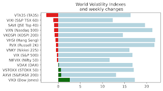
Weekly market report

Wall st delivered a mixed bag of news with VIX, VNKY, and VSTOXX and their underlying markets almost unchanged. VXD - volatility index based...